albumentations - fast image augmentation library 소개 및 사용법 Tutorial
안녕하세요, 최근 논문 리뷰 위주로 글을 작성해왔는데 얼마 전 알게 된 image augmentation library인 albumentations 가 생각보다 편하고 쓸만해서 간단히 소개드릴 예정입니다.
아! 추가로, 공부하다가 albumentations 라이브러리를 한글로 친절하게 설명해주시는 유튜브 강의 영상이 있어서 강의 영상을 보셔도 좋을 것 같습니다! 굉장히 상세하게 사용법을 설명해주시고 계십니다! ㅎㅎ 인용 허락해주셔서 감사합니다!!
What is albumentations?
저는 최근에는 주로 PyTorch를 사용하다 보니 image augmentation 등 imgae의 형태를 변환하여야 할 때, TorchVision에서 제공하고 있는 torchvision.transforms 를 주로 사용해왔습니다. Torchvision.transforms에도 자주 쓰이는 augmentation 기법들이 대부분 구현이 되어있어서 편하게 사용을 해왔고, custom augmentation이 필요한 경우 직접 구현해서 사용을 해왔습니다.
그러던 와중에 좀 더 다양한 augmentation을 지원하는 open source library가 없을까? 하고 찾아보던 중에 오늘 소개드릴 albumentations를 발견하였고 간단히 사용해본 결과, 처리 속도도 더 빠르고 기능도 다양하며 무엇보다 기존 torchvision.transforms으로 짜여져 있던 코드를 대체하는 것도 5분이 채 걸리지 않아서 이 albumentations를 앞으로 계속 사용해야겠다고 느꼈습니다.
Albumentations는 Albumentations: Fast and Flexible Image Augmentations 라는 이름으로 2020년 Information 저널에 출판이 되었으며 현재 6명의 연구자들이 관리 중이며 계속해서 새로운 기능들이 추가되고 있습니다.
다른 image augmentation 관련 library들과 비교해서 가장 큰 특징은 빠르다는 점이며, numpy, OpenCV, imgaug 등 여러 library(OpenCV 가 메인)들을 기반으로 optimization을 하였기 때문에 다른 library들보다 빠른 속도를 보여줍니다.
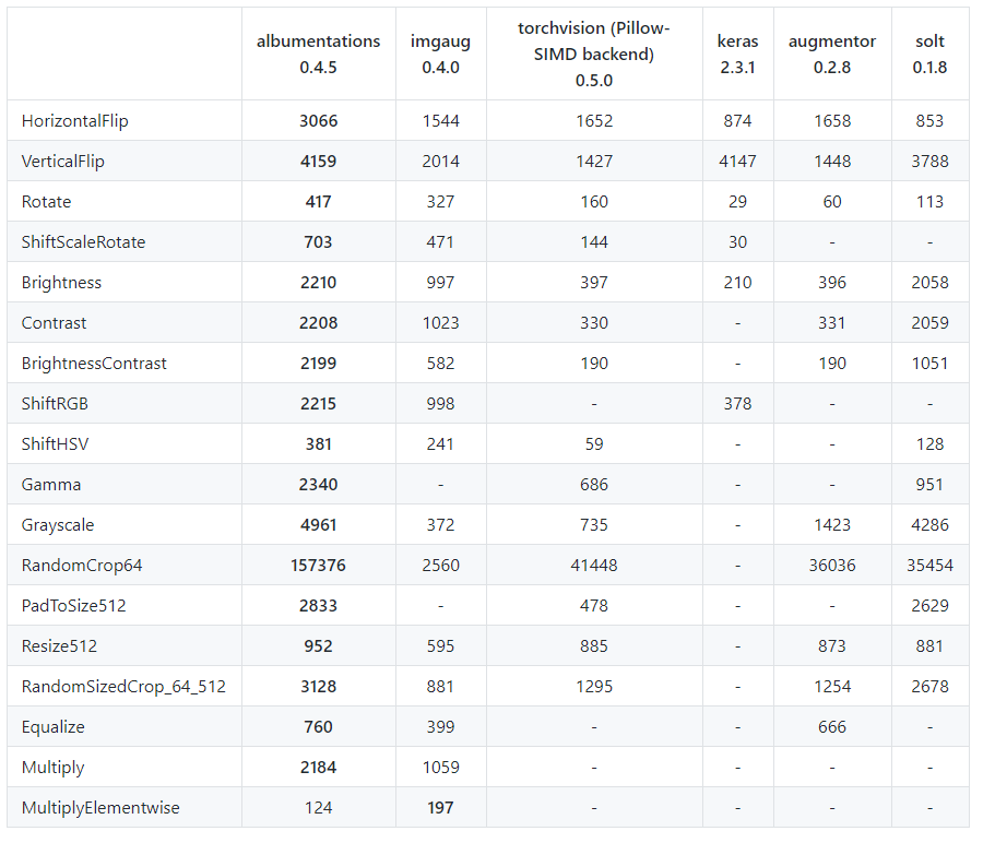
위의 표는 ImageNet의 validation set 2000장에 대해 Intel Xeon Platinum 8168 CPU로 test한 결과이며 표의 값은 single core에서 초당 처리되는 image의 수를 나타내고 있습니다. 거의 모든 transform에서 많게는 2배 이상 빠른 처리 속도를 보여주고 있습니다.
Albumentations 사용법 Tutorial
이제 albumentations의 사용 방법을 tutorial 형태로 소개 드리겠습니다. Tutorial 자료는 albumentations 팀에서 만든 tutorial notebook들을 기반으로 간단히 재구성해서 작성을 하였습니다. Albumentations의 기능들에 대한 소개 자료는 https://albumentations.readthedocs.io/ 에서 확인하실 수 있으며, 제가 참고한 tutorial notebook 들은 다음과 같습니다.
위의 참고 자료를 바탕으로 간단하게 예시를 준비해보았는데요, 제가 보여드리는 예시를 그대로 재현해보고 싶으신 분들은 해당 예제 를 이용하시면 됩니다. Google colab을 기반으로 간단하게 작성해보았습니다.
Google Colab에 Google Drive 연동
우선 저는 간단한 코드를 구현할 때 Colab을 자주 활용합니다. 무료로 jupyter notebook을 이용할 수 있고, GPU도 사용이 가능합니다. 예시로는 제 어릴적 사진 1장을 준비해보았습니다. (별다른 이유는 없습니다.. ㅎㅎ)
우선 사용하실 test image를 본인의 구글 드라이브에 업로드를 하신 뒤, Google Drive를 Colab에 연동을 하겠습니다. 또한 본 튜토리얼에서 사용할 library들도 import 해주겠습니다.
from PIL import Image
import cv2
import numpy as np
import time
import torch
import torchvision
from torch.utils.data import Dataset
from torchvision import transforms
import albumentations
from matplotlib import pyplot as plt

from google.colab import drive
drive.mount("/content/gdrive")
위의 코드 block을 실행하면 Go to this URL in a browser: 라는 메시지와 함께 URL이 생성됩니다. 해당 URL을 클릭하신 뒤 google 계정을 인증하면 코드가 생성됩니다. 이 코드를 복사해서 입력해주고 enter를 누르면 Google drive가 마운트 됩니다.
기존 TorchVision Data Pipeline
저는 평소에 PyTorch와 TorchVision을 통해 Data Loader를 구현해서 사용을 합니다. 튜토리얼을 위해 간단한 Dataset class를 만들고, image를 불러와서 약간의 transform을 적용하는 과정을 보여드리고, 이를 100번 반복한 뒤 평균 수행 시간을 측정해보았습니다.
class TorchvisionDataset(Dataset):
    def __init__(self, file_paths, labels, transform=None):
        self.file_paths = file_paths
        self.labels = labels
        self.transform = transform

    def __len__(self):
        return len(self.file_paths)

    def __getitem__(self, idx):
        label = self.labels[idx]
        file_path = self.file_paths[idx]

        # Read an image with PIL
        image = Image.open(file_path)

        start_t = time.time()
        if self.transform:
            image = self.transform(image)
        total_time = (time.time() - start_t)

        return image, label, total_time
우선 torch.utils.data에서 Dataset abstract class를 가져온 뒤, 이를 바탕으로 TorchVisionDataset Class를 만들었습니다. __getitem__ 을 통해 image를 불러온 뒤 transform을 적용시킬 예정입니다. 또한 transform의 시간 측정을 위해 time 함수를 이용해서 시간을 측정하였습니다.
torchvision_transform = transforms.Compose([
    transforms.Resize((256, 256)),
    transforms.RandomCrop(224),
    transforms.RandomHorizontalFlip(),
    transforms.ToTensor(),
])

torchvision_dataset = TorchvisionDataset(
    file_paths=["/content/gdrive/My Drive/test.png"],
    labels=[1],
    transform=torchvision_transform,
)
transform으론 image를 256x256으로 resize한 뒤 224x224 크기로 random하게 crop을 수행합니다. 그 뒤 50% 확률로 Horizontal flip을 적용하고 Tensor 형태로 변환을 시킬 예정입니다. 이 때 input으로 넣어주는 file path는 위와 같이 Google Drive에서 업로드하신 파일의 경로를 입력해주시면 됩니다.
total_time = 0
for i in range(100):
  sample, _, transform_time = torchvision_dataset[0]
  total_time += transform_time

print("torchvision time/sample: {} ms".format(total_time*10))

plt.figure(figsize=(10, 10))
plt.imshow(transforms.ToPILImage()(sample))
plt.show()
그 뒤, torchvision_dataset에서 1개의 sample을 꺼내는 과정에서 transform에 소요된 시간을 계산하고, 이를 100번 반복하여 평균적으로 몇 ms가 걸리는지 측정하였습니다. 또한 transform을 먹인 image도 시각화하였습니다.
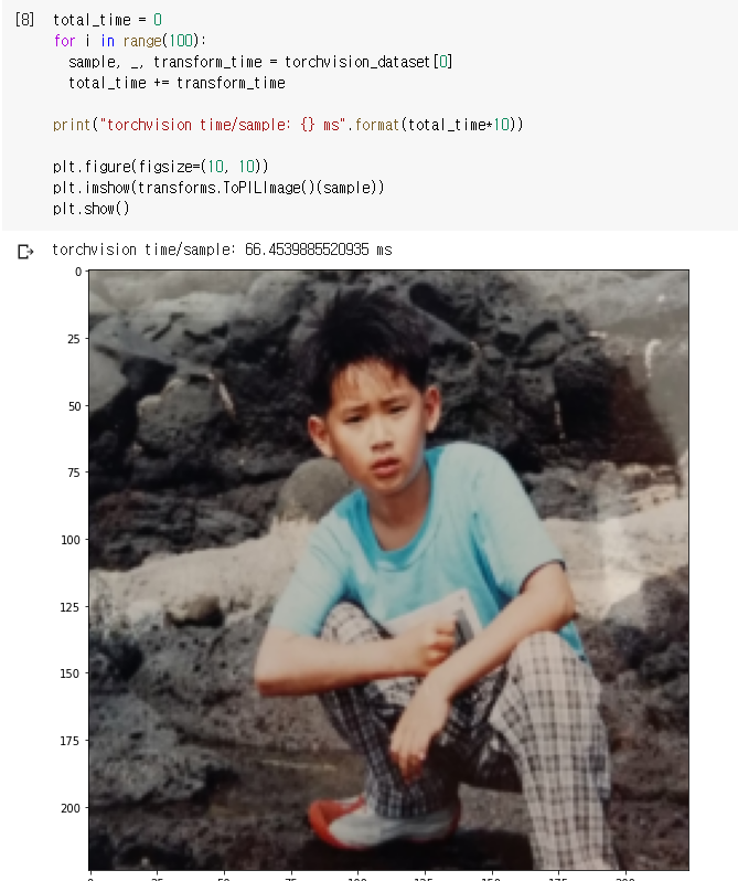
제가 정의한 Resize + RandomCrop + RandomHorizontalFlip 을 100번 반복한 결과 평균적으로 66.45ms 정도가 소요되었고, 100번째 transform을 먹인 image는 위의 그림과 같이 224x224 크기를 가지고, 아쉽게 Horizontal Flip은 적용되지 않은 것을 확인할 수 있습니다.
albumentations Data Pipeline
이제는 TorchVision으로 작성했던 Data Pipeline을 albumentations으로 거의 똑같이 구현을 해보겠습니다.
class AlbumentationsDataset(Dataset):
    """__init__ and __len__ functions are the same as in TorchvisionDataset"""
    def __init__(self, file_paths, labels, transform=None):
        self.file_paths = file_paths
        self.labels = labels
        self.transform = transform

    def __len__(self):
        return len(self.file_paths)

    def __getitem__(self, idx):
        label = self.labels[idx]
        file_path = self.file_paths[idx]

        # Read an image with OpenCV
        image = cv2.imread(file_path)

        # By default OpenCV uses BGR color space for color images,
        # so we need to convert the image to RGB color space.
        image = cv2.cvtColor(image, cv2.COLOR_BGR2RGB)

        start_t = time.time()
        if self.transform:
            augmented = self.transform(image=image)
            image = augmented['image']
	    total_time = (time.time() - start_t)
        return image, label, total_time
마찬가지로 torch.utils.data에서 Dataset abstract class를 바탕으로 AlbumentationsDataset class를 만들고, 비슷하게 구현을 해줍니다.
"""
torchvision_transform = transforms.Compose([
    transforms.Resize((256, 256)),
    transforms.RandomCrop(224),
    transforms.RandomHorizontalFlip(),
    transforms.ToTensor(),
])
"""

# Same transform with torchvision_transform
albumentations_transform = albumentations.Compose([
    albumentations.Resize(256, 256),
    albumentations.RandomCrop(224, 224),
    albumentations.HorizontalFlip(), # Same with transforms.RandomHorizontalFlip()
    albumentations.pytorch.transforms.ToTensor()
])
Torchvision.transforms 을 이용해서 구현했던 transform들을 albumentation의 transform을 이용해서 똑같이 구현해줍니다. 이 때, 약간의 차이가 있다면 torchvision의 RandomHorizontalFlip()과 같은 동작을 하는 함수가 albumentations에서는 HorizontalFlip()으로 구현이 되어있습니다.
# Same dataset with torchvision_dataset
albumentations_dataset = AlbumentationsDataset(
    file_paths=["/content/gdrive/My Drive/test.png"],
    labels=[1],
    transform=albumentations_transform,
)
total_time = 0
for i in range(100):
  sample, _, transform_time = albumentations_dataset[0]
  total_time += transform_time

print("albumentations time/sample: {} ms".format(total_time*10))

plt.figure(figsize=(10, 10))
plt.imshow(transforms.ToPILImage()(sample))
plt.show()
마찬가지로 하나의 image에 대해 transform을 적용시킨 뒤 100회 시간을 측정하여 평균을 낸 값과, transform이 적용된 image를 시각화하였습니다.
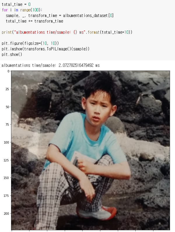
놀랍게도 torchvision을 사용하였을 때의 66.45ms보다 약 32배 빠른 2.07ms 정도가 소요되었습니다! 공식 문서에서 제공하고 있는 수치보다 더 큰 차이가 났는데 자세한 원인은 잘 모르겠습니다.. 아무튼 굉장히 빠르네요! 또한 이번엔 눈치채신 분도 계시겠지만 Horizontal Flip이 적용이 되었고(신발의 방향이 다릅니다), crop된 영역도 미세하기 차이가 있습니다.
albumentations 응용 사례
마지막으로 albumentation을 이용해서 복잡한 augmentation을 적용하는 예시를 보여드리겠습니다. 개인적으로 가장 유용하다고 느꼈던 OneOf 함수를 사용하여 구현을 하였습니다.
albumentations_transform_oneof = albumentations.Compose([
    albumentations.Resize(256, 256),
    albumentations.RandomCrop(224, 224),
    albumentations.OneOf([
                          albumentations.HorizontalFlip(p=1),
                          albumentations.RandomRotate90(p=1),
                          albumentations.VerticalFlip(p=1)
    ], p=1),
    albumentations.OneOf([
                          albumentations.MotionBlur(p=1),
                          albumentations.OpticalDistortion(p=1),
                          albumentations.GaussNoise(p=1)
    ], p=1),
    albumentations.pytorch.ToTensor()
])
Resize와 random crop까지는 같았고, OneOf 함수에서는 list 안의 있는 transform 들 중 하나를 random하게 가져옵니다. 또한 OneOf 함수 자체에도 확률을 부여할 수 있습니다. 만약 one of([…], p=0.5) 였다면, 0.5확률로는 해당 transform을 스킵하고, 위와 같이 3개의 transform을 list로 받았다면 각 transform들은 1/6 확률로 선택이 되는 것입니다.
저는 Horizontal Flip, Rotation, Vertical Flip 중에 하나를 random하게 선택하고, Blur, Distortion, Noise 연산 중 하나를 random하게 선택하여 보았습니다. 즉 3x3 = 9가지의 조합이 가능합니다.
albumentations_dataset = AlbumentationsDataset(
    file_paths=["/content/gdrive/My Drive/test.png"],
    labels=[1],
    transform=albumentations_transform_oneof,
)

num_samples = 5
fig, ax = plt.subplots(1, num_samples, figsize=(25, 5))
for i in range(num_samples):
  ax[i].imshow(transforms.ToPILImage()(albumentations_dataset[0][0]))
  ax[i].axis('off')
위에서 정의한 transform을 5번 적용한 결과는 다음과 같습니다.

왼쪽부터 차례대로 rotation 180, rotation 360, horizontal flip, vertical flip, horizontal flip이 적용이 되었으며, 각 이미지마다 서로 다른 distortion 함수가 적용이 되고 있습니다.
제가 사용한 transform 외에도 굉장히 다양한 transform이 존재하니 공식 문서 를 참고하셔서 여러가지 augmentation 기법들을 활용하시기 바랍니다!
결론
이번 포스팅에서는 image augmentation library인 albumentations에 대해 간단하게 소개를 드리고, 간단한 예제를 통해 사용 방법을 소개드렸습니다. 1장의 image로 실험을 하긴 했지만 굉장히 큰 폭의 속도 향상이 있었으며, 다양한 augmentation transform들을 지원하고 있고, TorchVision 으로 짜여진 코드에서 쉽게 대체가 가능하기 때문에 많이들 사용하시길 권장드립니다. 감사합니다!