Shake-Shake Regularization Review & TensorFlow code implementation
안녕하세요, 이번 포스팅에서는 이미지 인식 분야에서 보편적으로 적용되는 데이터 증강 기법을 소개 드리고, 관련된 내용 중 최신 논문에서 사용된 Shake-Shake 기법을 소개 드리려고 합니다. 데이터 증강 기법은 전부터 잘 알려져 있는 방법들이 많기 때문에 간단하게 다루고, 비교적 관련 글이 적은 최신 논문의 내용 위주로 Tensorflow 구현 코드와 함께 설명을 드릴 예정입니다. 혹시 글이나 코드를 보시다가 잘 이해가 되지 않는 부분은 편하게 댓글에 질문을 주시면 답변 드리겠습니다!!
- 다음과 같은 사항을 알고 계시면 더 이해하기 쉽습니다.
- 딥러닝에 대한 전반적인 이해
- Python 언어 및 Tensorflow 프레임워크에 대한 이해
- 이번 포스팅에서 구현한 Shake-Shake의 경우 Image Classification 성능을 측정하였으며, 실제 논문에서 사용한 프레임워크(torch)와 다른 프레임워크를 사용하였기 때문에 완벽한 재현이 되지 않을 가능성이 있습니다.
- 이번 포스팅에서도 지난 Classification 구현체의 포스팅의 구조인 데이터셋(Data set), 성능 평가(Performance evaluation), 러닝 모델(Learning model), 러닝 알고리즘(Learning algorithm) 4 요소를 구현하였으며, 일부 추가된 부분 위주로 설명합니다.
- 전체 구현체 코드는 수아랩의 GitHub 저장소 에서 자유롭게 확인 가능합니다.
- 이번 포스팅에서 다룬 데이터셋인 CIFAR-10은 keras의 helper module을 통해 자동으로 불러오도록 되어있으며, 하드디스크 혹은 SSD에 최소 200MB의 용량을 확보해두시면 좋습니다.
서론 (Data augmentation이란?)
이미지 인식 분야에서 데이터의 개수를 증강시키는 data augmentation 기법은 성능에 큰 영향을 미치고 있습니다. 일반적으로 딥러닝의 데이터의 개수는 많으면 많을 수록 좋다고 알려져있습니다. 만약 가지고있는 데이터의 개수가 적은 상황에서 가장 쉽게 취할 수 있는 행동은 데이터를 추가로 취득하는 작업입니다. 하지만 현실적으로 판단해보면 시간과 인력 등이 필요하고, 이들이 갖춰진다고 해도 데이터를 추가로 취득하기가 어려운 경우가 많습니다. 그럴 때 인위적으로 데이터의 개수를 늘려주면 데이터를 추가로 취득한 효과를 볼 수 있습니다.
딥러닝을 공부하시는 분들, 실제로 사용을 하시는 분들은 필연적으로 augmentation 기법을 접해 보셨을 것입니다. 서론에서는 주로 사용되는 데이터 증강 기법들을 간단하게 소개 드리겠습니다.
일반적으로 데이터 증강은 하나의 이미지를 통해 여러 장의 이미지로 개수를 늘리는 방법을 의미하며, 원본 이미지를 어떻게 변형시키는지에 따라 기법이 달라집니다. 대표적인 기법들을 소개해드리면 다음과 같습니다.
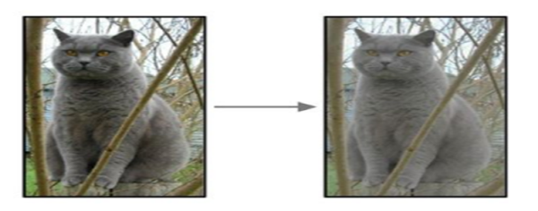
- 이미지 반전 (Flip)
가장 자주 사용되는 방법이며 말 그대로 이미지 자체를 좌우 혹은 상하로 반전시키는 것을 의미합니다.
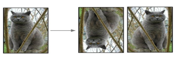
- 이미지 회전 (Rotation)
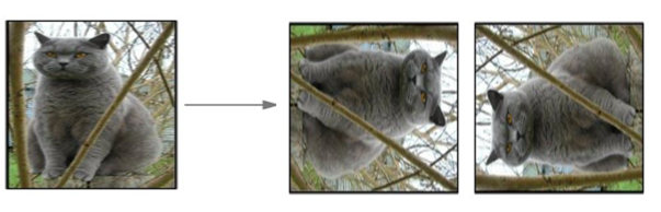
마찬가지로 가장 자주 사용되는 방법이며 말 그대로 이미지를 회전 시키는 방법이며 주로 시계 방향 혹은 반 시계 방향으로 90, 180, 270도 회전을 시키며, 간혹 데이터의 개수를 많이 늘려야 하는 경우에는 30도, 45도 등으로 회전을 시키고 빈 공간에는 0으로 채워 넣는 방식도 사용합니다.
- 이미지 자르기 (Crop)
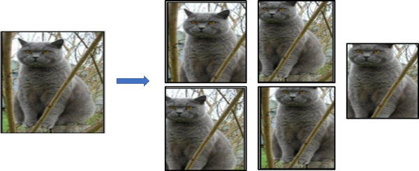
주로 고정된 입력 크기를 갖는 CNN에서 사용되는 방법으로, 하나의 이미지를 규칙에 맞게, 혹은 random으로 자르는 방법을 의미합니다. 예를 들어 AlexNet 논문에서는 256 x 256 크기의 이미지에서 좌측 상단, 우측 상단, 좌측 하단, 우측 하단, 중앙 부분에서 5장의 227 x 227 패치를 잘라내서 1장으로부터 5장의 이미지를 얻는 방법을 사용하였습니다. 패치를 자르는 위치를 random 하게 가져갈 수도 있습니다.
또한 위에서 서술한 것처럼 큰 이미지에서 작은 이미지로 잘라내는 방식 외에도, 잘라낸 이미지(227 x 227)를 원본 이미지(256 x 256)의 크기로 resize하여 사용하기도 합니다.
- 그 외의 기법들
위에서 소개드린 기법 외에도 여러 기법이 사용됩니다. 주로 노이즈를 주입하는 방식과 영상처리 기법을 통해 이미지를 변형시키는 방법 등이 있습니다.
Color Jittering이라 불리는 방법이 주된 노이즈 주입 기법인데, 이미지의 픽셀 값(RGB)에 랜덤하게 노이즈를 주입할 수 도 있고, 복잡하게는 학습 이미지들에 대해 주성분 분석 기법인 PCA를 수행한 뒤, 픽셀 값(RGB)에 변화를 주는 방법이 있습니다.
영상 처리 기법은 이미지에 랜덤하게 검은 점과 흰 점들을 더해주는 Salt and pepper noise 기법을 사용하거나 이미지를 Blur시키는 기법 등 픽셀 단위로 이미지를 변형시키는 방법, Edge 영역에 강조를 두는 방법 등 여러 방식으로 응용될 수 있습니다.
가장 중요한 점은 데이터셋의 특징에 따라 사용 가능한 증강 기법도 다르기 때문에 사용하실 때 데이터의 성질을 변화시키지 않는 선에서 사용해야 한다는 점입니다.
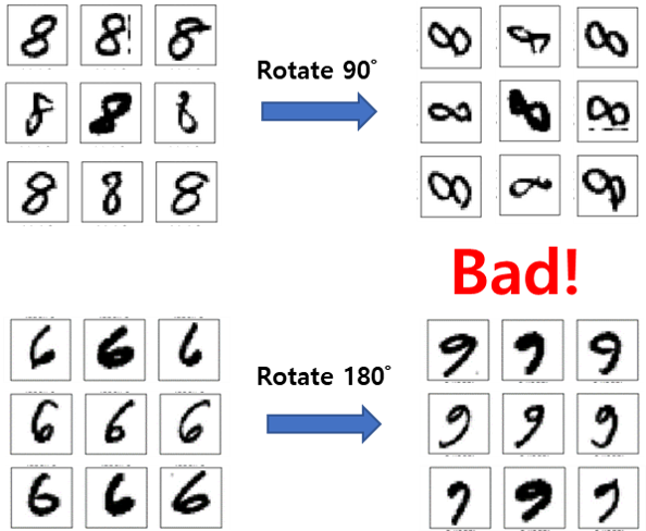
예를 들어 숫자 0~9를 인식하는 MNIST 데이터셋을 예로 들어보면, 숫자 8의 경우 좌우, 상하로 반전을 시켜도 숫자 8의 성질이 유지되지만, 90도 회전을 시키면 숫자 8의 성질을 갖지 않게 됩니다. 마찬가지로 숫자 6의 경우에도 180도 회전을 시키면 숫자 9의 성질을 갖게 됩니다. 그러므로 데이터의 성질에 따라 적용할 기법을 다르게 가져가야 합니다.
논문 소개 (Shake-Shake regularization)
이번 포스팅에서 소개드릴 Shake-Shake regularization 논문은 앞서 설명 드렸던 data augmentation 기법과 관련이 있습니다. 차이점은 일반적인 augmentation은 입력 이미지를 타겟으로 이루어지는 반면, Shake-shake 기법은 논문의 표현을 인용하면 “Internal Representations”에 augmentation 기법을 적용하겠다고 주장을 합니다. 아래의 그림이 이를 잘 설명해주고 있습니다.
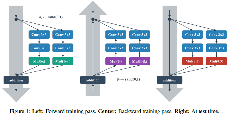
정말 간단하게 표현을 하자면 입력 이미지 단계에서 증강시키는 것이 아니고 내부 표현, 즉 Feature map 단계에서, 정확하게는 학습 과정에서 Gradient를 증강시킨다고 이해하시면 될 것 같습니다. Figure 1의 왼쪽 그림과 같이 같은 구조를 갖는, 본 포스팅에서는 Shake branch라 부르는 2개의 residual branch가 같은 구조를 가지고, 연산을 거친 후에 feature map에 0과 1 사이의 임의의 스칼라 값인 α, 1- α를 곱하여 더한 feature map을 사용합니다. 그 후 가운데 그림을 보면 Back propagation 단계에서도 임의의 스칼라 값을 곱해주는 방식으로 증강을 하고 있습니다. Randomness를 학습 단계에 주입함으로써 Regularization 효과도 얻고, 논문의 표현을 인용하면 “Stochastic blend” 효과를 얻을 수 있다고 합니다.
다소 실험적인 방법론이라 왜 이러한 시도가 있었는지 잘 이해가 되지 않을 수 있습니다. 더 깊은 이해를 위해서는 선행 연구들을 살펴보아야 합니다. 하지만 이번 포스팅에는 선행 연구들도 정리하면 글이 너무 길어지고 요점을 제대로 짚지 못할 것 같아 간단하게 키워드와 그림으로 소개 드리겠습니다.
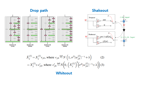
우선 FractalNet의 drop-path(Larsson et al., 2016) 방식은 Residual branch 중 일부를 임의로 0을 곱하도록 하는 방식을 사용하였고, 이 외에도 dropout과 유사한 방식을 사용한 shakeout(Kang et al., 2016), whiteout(Yinan et al., 2016) 등이 있으니 관심이 있으신 분들은 참고하시면 될 것 같습니다.
다시 본론으로 돌아와서, 논문에서 위의 내용들을 간단하게 서론에서 소개를 한 뒤 본론에서는 CIFAR-10과 CIFAR-100에 대해서 각각의 자세한 구현 내용, 실험 결과를 서술하고 있습니다. 이번 포스팅에서는 CIFAR-10 데이터셋에 대해서만 구현을 하였지만 혹 CIFAR-100에 대해서 실험을 하고싶으신 분들도 일부 수정만 하시면 되기 때문에 큰 어려움은 없을 것으로 예상됩니다.
우선 전체 CNN 아키텍처는 ResNet을 기반으로 만들어졌습니다. ResNet은 다들 많이 들어 보셨을 것으로 생각합니다. 혹시 처음 들어 보신 분들은 아마 간단한 검색을 통해 찾아보실 수 있을 것입니다. CIFAR-10에서 기본으로 삼는 base network는 26 2x32d ResNet이란 이름을 가지고 있는데요, 26은 전체 layer의 개수(depth)를 의미하고, 2는 residual branch의 개수, 32는 첫 residual block의 filter의 개수(width)를 의미합니다. 일반적으로 filter의 가로 세로를 표현할 때 3x3 convolutional filter를 예로 들면 “width=3, height=3인 filter다!” 고 생각할 수 있는데, 이 논문에서는 filter의 개수를 width로 표현을 해서 그 표현을 그대로 사용하였습니다. 논문에서는 depth와 residual branch의 개수는 고정하고, width 값을 32, 64, 96 등으로 조절을 하며 실험 결과를 제시합니다.
내부 구조는 다소 복잡하게 구성이 되어있습니다. 전체 26개의 layer 중에 첫 3x3 convolution layer와 마지막 fully-connected layer를 제외한 24개의 layer는 3개의 stage로 구성되고, 각 stage는 4개의 block으로 구성 되어있는 계층적인 구조로 구성이 되어있습니다. 글로만 설명을 하면 굉장히 복잡하기 때문에 그림을 준비하였습니다.
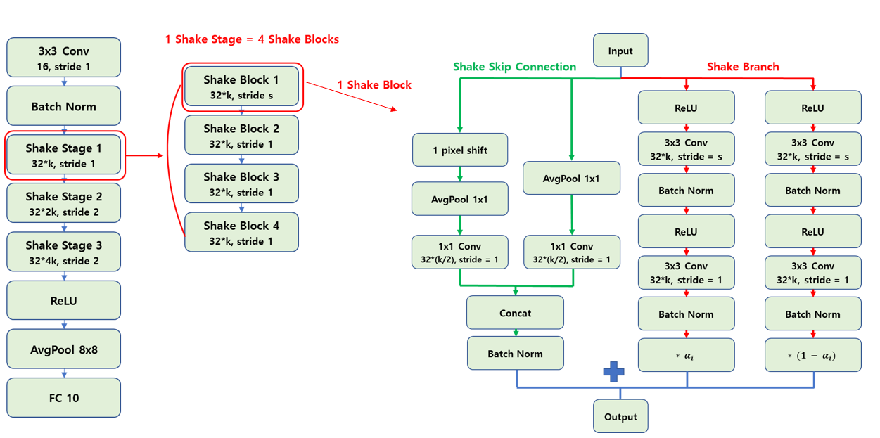
일단 그림의 notation은 Conv, shake stage, shake block 등의 연산 이름 아래의 숫자는 해당 연산을 거쳐 나오는 output feature map의 channel수를 의미하고 stride는 convolution 연산의 stride를 의미합니다. 예를 들어 3x3 Conv 16, stride 1은 3x3 Convolution 필터를 통해 16 채널을 갖는 feature map을 출력하는 것을 의미합니다.
첫 레이어와 마지막 레이어를 제외한 몸통 부분은 3개의 shake stage 로 구성이 되어있고, 매 stage마다 출력되는 feature map의 channel 수가 2배가 됩니다. 또한 첫번째 stage만 stride가 1이고 나머지 stage는 stride가 2인데, 이는 통상적으로 사용되는 CNN에서 max pooling등의 pooling을 거쳐 feature map의 가로 세로 크기가 절반으로 줄어드는 과정을 pooling 대신 strided convolution 연산으로 대체한 것을 의미합니다. 딥러닝의 기술은 하루하루 빠르게 변하고 있으므로 이 글을 작성하고 있는 시점(2018년 6월)을 기준으로 말씀드리면 최근에는 pooling 대신 stride를 넣은 convolution 연산이 좋은 성능을 보이는 경우가 많아 자주 사용되고, 본 논문에서도 그렇게 사용한 것으로 판단됩니다.
또한 각 shake stage는 4개의 shake block으로 구성이 되어있고, 첫번째 block에서만 stride 값이 해당 stage의 stride 값을 사용하고 나머지 block은 stride가 1로 고정이 되는 구조를 보입니다. 각 shake block은 이번 포스팅에서는 shake branch라 부르는 2개의 residual branch와, shake skip connection이라 부르는 skip connection layer로 구성되어 있습니다.
shake branch는 위 그림의 shake block 구조도에서 빨간색 선으로 연결되어있는 부분을 의미하며 동일한 연산을 2방향으로 나뉘어서 수행한 뒤 각 결과에 각각 α, 1- α를 곱하여 결과를 출력하는 구조를 가지고 있습니다. 내부 연산은 ReLU와 Conv, Batch norm이 반복해서 사용되는 구조를 보입니다.
shake skip connection은 위 그림의 shake block 구조도에서 초록색 선으로 연결되어있는 부분을 의미합니다. ShakeNet에서는 첫 번째 shake_block을 제외하고는 입력 feature map과 출력 feature map의 채널 수가 같은데, 이 경우 기존에 저희가 잘 알고있던 skip connection 구조를 그대로 따릅니다. 채널 수가 다른 경우에는 Shake branch처럼 2방향으로 나뉘어서 연산을 수행한 뒤 하나로 합쳐지는 다소 특이한 방식의 skip connection 구조를 사용합니다. 각각 1x1 average pooling와 1x1 convolution 연산은 동일하지만, 약간의 변화를 주기 위해 둘 중 하나의 입력을 우측 하단 방향으로 1 pixel씩 shift를 하고 빈 자리를 0으로 채워 넣는 padding 과정을 거치는 독특한 구조를 가지고 있습니다.
그 뒤 결과를 concatenation하고 Batch normalization을 거친 결과와, shake branch를 거쳐 나온 결과를 element-wise로 더하여 하나의 shake block의 출력을 구하게 됩니다. 이렇게 되면 하나의 shake block을 거친 것이고, 이렇게 4개의 shake block을 거치고서야 하나의 shake stage를 거치게 되는 것입니다. 3개의 shake stage를 거치면 전체 ShakeNet의 몸통 부분을 전부 수행하게 됩니다.
그래서 CIFAR-10의 base network인 26 2x32d ResNet의 depth 값인 26은 첫 3x3 convolution layer와 마지막 fully-connected layer에 3개의 shake stage, 각 stage는 4개의 shake block, 각 block에는 2개의 convolution layer로 이루어져 있어 3 * 4 * 2 = 24개의 layer로 구성이 되어있는 것을 의미하게 됩니다. 이번 포스팅에서는 depth 값이 26인 경우만 다루지만, 혹시 depth를 늘리거나 줄이고 싶으신 분은 shake stage의 개수를 조절하거나, shake block의 개수를 조절하거나 각 block안의 연산들을 조절하시면 depth 값을 줄이거나 늘릴 수 있을 것입니다.
다음 설명드릴 부분은 shake branch의 randomness를 주는 스칼라 값인 α, 1- α를 어떻게 처리할 지에 대한 부분입니다. 본 논문에서는 다양한 실험 셋팅을 통해 최적의 조합을 찾아냈습니다.
- Forward pass
- Even / Shake
- Backward pass
- Even / Shake / Keep
- Mini-batch update rule
- Image / Batch
우선 Forward pass에서는 α 값을 0.5로 고정하는 “Even” 방식과, random 스칼라 값을 사용하는 “Shake” 방식으로 나뉩니다. Backward pass에서는 마찬가지로 β 값을 0.5로 고정하는 “Even” 방식과 random 스칼라 값을 사용하는 “Shake” 방식, forward pass에서 사용했던 α 값을 그대로 β 값으로 사용하는 “Keep” 방식으로 나뉩니다. 마지막으로 Mini-batch를 update해줄 때 각 배치의 이미지마다 다른 α, β 값을 사용하는 “Image” 방식과 하나의 mini-batch에서 같은 α, β 값을 사용하는 “Batch” 방식으로 나뉩니다.
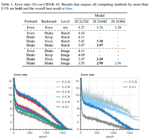
Table 1은 3가지 옵션을 바꿔가며 CIFAR-10 데이터셋에 대하여 측정한 결과를 보여주고 있습니다. 가장 성능이 좋은 조합은 “Shake”-“Shake”-“Image” 조합이며 결과를 각 옵션마다 분석을 해보면 다음과 같습니다.
- Forward pass
- “Even”을 사용하는 것보다 “Shake”를 사용하는 것이 성능이 좋음.
- Backward pass
- “Shake” > “Even” > “Keep” 순서로 성능이 좋음.
- Mini-batch update rule
- “Batch”를 사용하는 것보다 “Image”를 사용하는 것이 성능이 좋음.
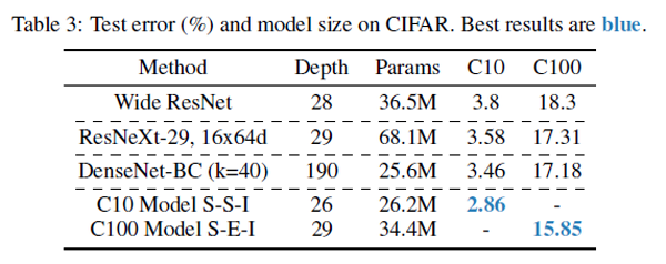
Shake-Shake regularization 기법을 사용하였을 때, 기존의 State-Of-The-Art(SOTA) 성능을 보인 다른 network들과 비교를 한 실험 결과도 있는데, 기존의 Wide ResNet, DenseNet 등에 비해 CIFAR-10, CIFAR-100에서 모두 좋은 성능을 보이는 것을 확인할 수 있습니다.
논문의 결과 다음 부분에는 딥러닝 논문에서 흔히 볼 수 있는 제안한 방법이 잘되는 이유를 관찰하고, 여러 셋팅을 바꿔가며 분석한 내용이 제시되어 있습니다.
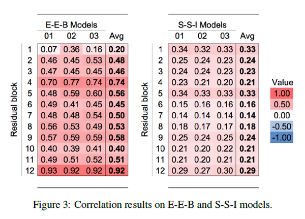
첫째론 Residual branch간 correlation을 분석하였습니다. 2개의 residual branch의 출력 feature map을 일렬로 펼친 뒤, 두 vector간의 covariance를 계산하여 correlation을 구하였습니다. 앞선 Table 1의 결과들 중 성능 차이가 컸던 “Even”-“Even”-“Batch” 조합(이하 E-E-B)과 “Shake”-“Shake”-“Image” 조합(이하 S-S-I) 간의 비교를 진행하였습니다. 그 결과, 성능이 좋았던 S-S-I 모델이 E-E-B 모델에 비해 대부분의 block에서 correlation이 작게 측정되었음을 관찰할 수 있고, 이는 E-E-B 모델에서 regularization 효과가 더 컸음을 보여주고 있습니다.
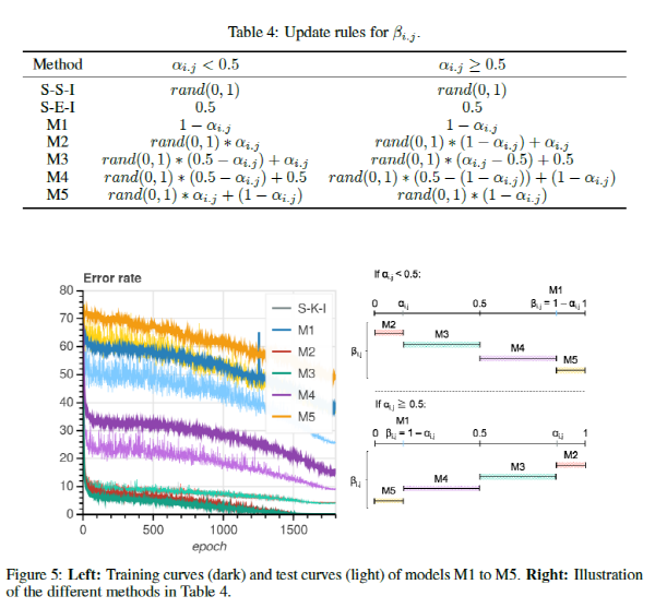
두번째 실험 결과로는 backward pass에서 사용하는 β 값을 α 값으로부터 어떻게 변화를 시키는지에 따라 성능이 어떻게 바뀌는지를 실험적으로 관찰한 결과를 제시하고 있습니다. Random 스칼라 값을 사용하는 “Shake”와 0.5를 사용하는 “Even” 외에 Table 4에 나와있는 것처럼 5가지 방법으로 β를 정의한 뒤 각 Method에 대해 성능을 측정하였습니다. 실험 결과 대체로 table 4의 M1, M5와 같이 β 가 α와 멀리 떨어져 있을수록 성능이 낮은 것을 알 수 있습니다. 혹시 S-S-I 방식보다 약간이라도 더 높은 성능을 달성하고 싶을 때, β 값을 어떻게 정하면 될지에 대한 약간의 가이드를 제시해주고 있다고 이해하시면 될 것 같습니다.
마지막 실험 결과로는 ShakeNet에서 skip connection을 제거하거나 Batch normalization을 제거하는 실험을 진행하였습니다. (솔직히 이 부분은 논문의 분량을 늘리기 위해 진행한 것이 아닐까 개인적으로 생각해봅니다.) 요약하자면 skip connection을 제거하면 약 1% 포인트의 성능 저하가 있지만 그럭저럭 잘 동작할 수 있음을 실험적으로 보였고, Batch normalization을 제거하면 성능 저하도 크고 모델이 발산할 수도 있음을 실험적으로 보였습니다. 결론은 Skip connection도 사용하고, Batch normalization도 사용하자! 입니다.
여기까지가 논문에 대한 소개였습니다. 요약하자면 ResNet을 기반으로 feature map 레벨, 정확하게는 gradient 레벨에서 augmentation을 하는 것과 같은 효과를 보기 위해 Shake-Shake 기법을 제안하였고, 그 결과 CIFAR 데이터셋에 대해 SOTA 성능을 달성하였다! 정도로 내용을 압축할 수 있을 것 같습니다.
이 논문을 읽고, 구현을 해본 입장에서 드는 생각은 이 방법이 CIFAR 데이터셋이 아닌 다른 데이터셋에서도 성능을 측정하면 어떤 결과가 나올지, 다른 데이터셋에서도 좋은 성능이 보장이 되는지 등의 내용이 논문에 추가가 되었으면 하는 아쉬움이 들었습니다. 다음에 설명드릴 부분에서는 Tensorflow로 구현한 구현체에 대한 설명이 포함되어 있는데, 혹시 CIFAR 데이터가 아닌 다른 데이터에 대해서도 실험을 하고 싶은 분은 이 코드를 사용하시고 데이터를 불러오는 부분, 모델의 입출력 크기 등 코드의 일부를 수정하시면 쉽게 사용이 가능할 것입니다.
본론 (실험 셋팅 + 코드 + 설명)
(1) 데이터셋: CIFAR-10
본 논문에서는 성능 검증을 위해 CIFAR-10, CIFAR-100 데이터셋에 대해 실험을 진행하였습니다. 하지만 이번 포스팅에서는 편의상 CIFAR-10 데이터셋에 대해서만 실험을 진행하였습니다.
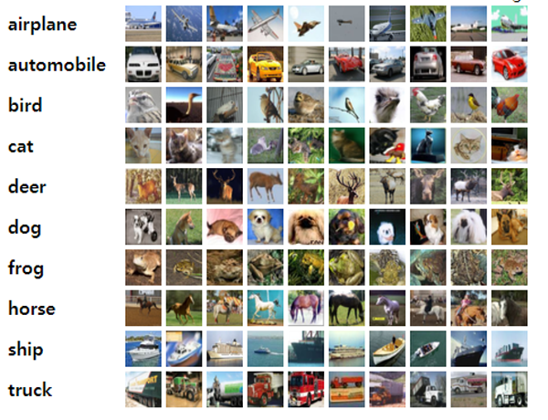
우선 CIFAR-10 데이터셋은 CIFAR(Canadian Institute For Advanced Research) 라는 기관에서 머신러닝과 컴퓨터비전 분야에서 사용할 수 있도록 수집한 이미지 데이터셋을 의미합니다. 뒤의 숫자 10은 class의 개수가 10개인 것을 의미하고, 100은 class 개수가 100개인 것을 의미합니다.
이미지는 총 60,000장으로 구성되어 있고 50,000장은 학습에, 10,000장은 테스트에 사용하도록 나뉘어져 있습니다. 이미지는 32x32에 RGB 3채널로 비교적 작은 크기를 갖고 있고, class는 “airplane”, “cars”, “birds”, “cats”, “deer”, “dogs”, “frogs”, “horses”, “ships”, “trucks” 로 구성이 되어있습니다.
dataset.cifar10 모듈
dataset.cifar10 모듈은 데이터셋 요소에 해당하는 함수들과 클래스 정보를 담고 있습니다. 수아랩 기술블로그의 포스팅 에서 사용했던 코드를 기반으로 작성을 하였기 때문에 모든 코드를 설명하기보다는 달라진 부분 위주로 설명을 드리겠습니다.
read_CIFAR10_subset 함수
def read_CIFAR10_subset():
    """
    Load the CIFAR-10 data subset from keras helper module
    and perform preprocessing for training ResNet.
    :return: X_set: np.ndarray, shape: (N, H, W, C).
             y_set: np.ndarray, shape: (N, num_channels) or (N,).
    """

    # Download CIFAR-10 data and load data
    (x_train, y_train), (x_test, y_test) = load_data()

    y_train_oh = np.zeros((len(y_train), 10), dtype=np.uint8)
    for i in range(len(y_train)):
        y_train_oh[i, y_train[i]] = 1
    y_train_one_hot = y_train_oh

    y_test_oh = np.zeros((len(y_test), 10), dtype=np.uint8)
    for i in range(len(y_test)):
        y_test_oh[i, y_test[i]] = 1
    y_test_one_hot = y_test_oh

    x_train = x_train/255.0
    x_test = x_test/255.0

    cifar_mean = np.array([0.4914, 0.4822, 0.4465])
    cifar_std = np.array([0.2470, 0.2435, 0.2616])

    for i in range(len(x_train)):
        x_train[i] -= cifar_mean
        x_train[i] /= cifar_std

    for j in range(len(x_test)):
        x_test[j] -= cifar_mean
        x_test[j] /= cifar_std

    print('x_train shape : ', x_train.shape, end='\n')
    print('x_test shape : ', x_test.shape, end='\n')
    print('y_train_one_hot shape : ', y_train_one_hot.shape, end='\n')
    print('y_test_one_hot shape : ', y_test_one_hot.shape, end='\n')
    print('\nDone')

    return x_train, x_test, y_train_one_hot, y_test_one_hot
고맙게도 keras의 helper module을 통해 CIFAR-10 데이터셋을 불러오는 함수를 tensorflow에서 사용할 수 있어서 데이터를 불러오는 과정을 손쉽게 함수 하나로 처리할 수가 있습니다. 자동으로 50,000장의 학습 데이터 (x_train, y_train)와 10,000장의 검증 데이터 (x_test, y_test)로 나뉘어서 데이터를 불러온 뒤, One-hot encoding을 거쳐 label을 생성해냅니다.
cifar_augment 함수
def cifar_augment(images):
    """
    Perform data augmentation from cifar images.
    :param images: np.ndarray, shape: (N, C, H, W).
    :return: np.ndarray, shape: (N, C, H, W).
    """
    augmented_images = []
    for image in images:    # image.shape: (C, H, W)
	# horizontal flip with 0.5 probability
        reflection = bool(np.random.randint(2))
        if reflection:
             image = np.fliplr(image)

        # random cropping with padding
        image_pad = np.pad(image, ((4,4), (4,4), (0,0)), mode='constant')

        crop_x1 = random.randint(0, 8)
        crop_x2 = crop_x1 + 32
        crop_y1 = random.randint(0, 8)
        crop_y2 = crop_y1 + 32

        image_crop = image_pad[crop_x1:crop_x2, crop_y1:crop_y2]

        augmented_images.append(image_crop)

    return np.stack(augmented_images)    # shape: (N, C, H, W)
CIFAR-10 데이터셋에서 성능 향상에 도움이 된다고 알려져있는 기법을 사용하였습니다. 우선 50% 확률로 좌우 반전을 한 뒤, 상하좌우에 4픽셀씩 패딩을 하고 임의의 32x32 크기의 패치를 추출하는 Random Crop 기법도 적용하였습니다. 서론에 설명드린 부분을 이해하신 분들이라면 쉽게 따라오실 수 있을 것이라 생각합니다. 또한 test시에는 따로 augmentation을 수행하지 않았습니다.
DataSet 클래스
DataSet 클래스에서 달라진 점은 지난 번 AlexNet에서는 data augmentation을 수행할 때 256x256 이미지로부터 227x227 크기의 패치(patch)를 추출하는 augmentation을 사용하였는데 이번 포스팅에서는 cifar_augment 함수로 대체를 하였습니다.
class DataSet(object):
    def __init__(self, images, labels=None):
        """
        Construct a new DataSet object.
        :param images: np.ndarray, shape: (N, H, W, C).
        :param labels: np.ndarray, shape: (N, num_classes) or (N,).
        """
        if labels is not None:
            assert images.shape[0] == labels.shape[0], (
                'Number of examples mismatch, between images and labels.'
            )
        self._num_examples = images.shape[0]
        self._images = images
        self._labels = labels    # NOTE: this can be None, if not given.
        self._indices = np.arange(self._num_examples, dtype=np.uint)    # image/label indices(can be permuted)
        self._reset()

    def _reset(self):
        """Reset some variables."""
        self._epochs_completed = 0
        self._index_in_epoch = 0

    @property
    def images(self):
        return self._images

    @property
    def labels(self):
        return self._labels

    @property
    def num_examples(self):
        return self._num_examples

    def next_batch(self, batch_size, shuffle=True, augment=True, is_train=True,
                   fake_data=False):
        """
        Return the next `batch_size` examples from this dataset.
        :param batch_size: int, size of a single batch.
        :param shuffle: bool, whether to shuffle the whole set while sampling a batch.
        :param augment: bool, whether to perform data augmentation while sampling a batch.
        :param is_train: bool, current phase for sampling.
        :param fake_data: bool, whether to generate fake data (for debugging).
        :return: batch_images: np.ndarray, shape: (N, h, w, C) or (N, 10, h, w, C).
                 batch_labels: np.ndarray, shape: (N, num_classes) or (N,).
        """

        start_index = self._index_in_epoch

        # Shuffle the dataset, for the first epoch
        if self._epochs_completed == 0 and start_index == 0 and shuffle:
            np.random.shuffle(self._indices)

        # Go to the next epoch, if current index goes beyond the total number of examples
        if start_index + batch_size > self._num_examples:
            # Increment the number of epochs completed
            self._epochs_completed += 1
            # Get the rest examples in this epoch
            rest_num_examples = self._num_examples - start_index
            indices_rest_part = self._indices[start_index:self._num_examples]

            # Shuffle the dataset, after finishing a single epoch
            if shuffle:
                np.random.shuffle(self._indices)

            # Start the next epoch
            start_index = 0
            self._index_in_epoch = batch_size - rest_num_examples
            end_index = self._index_in_epoch
            indices_new_part = self._indices[start_index:end_index]

            images_rest_part = self.images[indices_rest_part]
            images_new_part = self.images[indices_new_part]
            batch_images = np.concatenate((images_rest_part, images_new_part), axis=0)
            if self.labels is not None:
                labels_rest_part = self.labels[indices_rest_part]
                labels_new_part = self.labels[indices_new_part]
                batch_labels = np.concatenate((labels_rest_part, labels_new_part), axis=0)
            else:
                batch_labels = None
        else:
            self._index_in_epoch += batch_size
            end_index = self._index_in_epoch
            indices = self._indices[start_index:end_index]
            batch_images = self.images[indices]
            if self.labels is not None:
                batch_labels = self.labels[indices]
            else:
                batch_labels = None

        if augment and is_train:
            # Perform data augmentation, for training phase
            batch_images = cifar_augment(batch_images)
        else:
            # Don't perform data augmentation
            batch_images = batch_images

        return batch_images, batch_labels
(2) 성능 평가: 정확도
Classification에서 주로 사용되는 정확도(accuracy)를 성능 평가 척도로 사용하였습니다. Class의 개수가 10개이므로 각 class마다 얼마나 정확하게 예측했는지 Precision, Recall등을 측정할 수도 있지만 이번 포스팅에서는 전체 이미지에 대해서 단지 얼마나 정확하게 예측했는지에 대해서만 평가하였습니다.
성능 평가와 관련된 모듈들은 수아랩 기술블로그의 포스팅의 구현체와 달라진 점이 없으므로 따로 설명을 하진 않겠습니다. 혹시 궁금하신 분들은 이전 포스팅을 참고하시면 됩니다.
(3) 러닝 모델: ShakeNet (ResNet-26 with shake-shake)
이번 포스팅에서 가장 중요하게 다룬 부분이 바로 이 러닝 모델 부분입니다. 만약 논문만 읽고 이해가 잘 되지 않으신 분들은 이 코드들을 한 줄 한 줄 천천히 읽어보면서 이해를 하시는 것을 추천 드립니다.
models.layers 모듈
models.layers 모듈에서는 batch normalization을 수행하는 batch_norm 함수가 추가가 되었고, 그 외에 convolution layer, fully-connected layer 등은 기존의 것들을 그대로 사용하였습니다. 다만 달라진 점은 batch normalization을 수행하기 때문에 bias는 사용하지 않습니다. 또한 가중치(weight) 초기화(initialize)는 이전 포스팅의 방식과는 다르게 Xavier initialization 기법을 사용하였습니다.
import tensorflow as tf

def weight_variable(shape):
    """
    Initialize a weight variable with given shape,
    by Xavier initialization.
    :param shape: list(int).
    :return weights: tf.Variable.
    """
    weights = tf.get_variable('weights', shape, tf.float32, tf.contrib.layers.xavier_initializer())

    return weights

def bias_variable(shape, value=1.0):
    """
    Initialize a bias variable with given shape,
    with given constant value.
    :param shape: list(int).
    :param value: float, initial value for biases.
    :return biases: tf.Variable.
    """
    biases = tf.get_variable('biases', shape, tf.float32,
                             tf.constant_initializer(value=value))
    return biases

def conv2d(x, W, stride, padding='SAME'):
    """
    Compute a 2D convolution from given input and filter weights.
    :param x: tf.Tensor, shape: (N, H, W, C).
    :param W: tf.Tensor, shape: (fh, fw, ic, oc).
    :param stride: int, the stride of the sliding window for each dimension.
    :param padding: str, either 'SAME' or 'VALID',
                         the type of padding algorithm to use.
    :return: tf.Tensor.
    """
    return tf.nn.conv2d(x, W, strides=[1, stride, stride, 1], padding=padding)

def max_pool(x, side_l, stride, padding='SAME'):
    """
    Performs max pooling on given input.
    :param x: tf.Tensor, shape: (N, H, W, C).
    :param side_l: int, the side length of the pooling window for each dimension.
    :param stride: int, the stride of the sliding window for each dimension.
    :param padding: str, either 'SAME' or 'VALID',
                         the type of padding algorithm to use.
    :return: tf.Tensor.
    """
    return tf.nn.max_pool(x, ksize=[1, side_l, side_l, 1],
                          strides=[1, stride, stride, 1], padding=padding)

def conv_layer_no_bias(x, side_l, stride, out_depth, padding='SAME'):
    """
    Add a new convolutional layer.
    :param x: tf.Tensor, shape: (N, H, W, C).
    :param side_l: int, the side length of the filters for each dimension.
    :param stride: int, the stride of the filters for each dimension.
    :param out_depth: int, the total number of filters to be applied.
    :param padding: str, either 'SAME' or 'VALID',
                         the type of padding algorithm to use.
    :return: tf.Tensor.
    """

    in_depth = int(x.get_shape()[-1])

    filters = weight_variable([side_l, side_l, in_depth, out_depth])

    return conv2d(x, filters, stride, padding=padding)

def fc_layer(x, out_dim, **kwargs):
    """
    Add a new fully-connected layer.
    :param x: tf.Tensor, shape: (N, D).
    :param out_dim: int, the dimension of output vector.
    :param kwargs: dict, extra arguments, including weights/biases initialization hyperparameters.
        - biases_value: float, initial value for biases.
    :return: tf.Tensor.
    """
    biases_value = kwargs.pop('biases_value', 0.1)
    in_dim = int(x.get_shape()[-1])

    weights = weight_variable([in_dim, out_dim])
    biases = bias_variable([out_dim], value=biases_value)
    return tf.matmul(x, weights) + biases

def batch_norm(x, is_training, momentum=0.9, epsilon=0.00001):
    """
    Add a new batch-normalization layer.
    :param x: tf.Tensor, shape: (N, H, W, C).
    :param is_training: bool, train mode : True, test mode : False
    :return: tf.Tensor.
    """
    x = tf.layers.batch_normalization(x, momentum=momentum, epsilon=epsilon, training=is_training)
    return x
models.nn 모듈
models.nn 모듈은, 컨볼루션 신경망을 표현하는 클래스를 담고 있습니다.
ConvNet 클래스
models.nn 모듈에서 ConvNet 클래스는 크게 달라진 부분이 없고 단지 위에서 서술한 것처럼 augmentation 여부에 따라 약간의 수정이 있었습니다.
ShakeNet 클래스
class ShakeNet(ConvNet):
    """ShakeNet class."""

    def _build_model(self, **kwargs):
        """
        Build model.
        :param kwargs: dict, extra arguments for building ShakeNet.
            - batch_size: int, the batch size.
        :return d: dict, containing outputs on each layer.
        """
        d = dict()    # Dictionary to save intermediate values returned from each layer.
        batch_size = kwargs.pop('batch_size', 128)
        num_classes = int(self.y.get_shape()[-1])

        # input
        X_input = self.X

        # first residual block's channels (26 2x32d --> 32)
        first_channel = 32

        # the number of residual blocks (it means (depth-2)/6, i.e. 26 2x32d --> 4)
        num_blocks = 4

        # conv1 - batch_norm1
        with tf.variable_scope('conv1'):
            d['conv1'] = conv_layer_no_bias(X_input, 3, 1, 16, padding='SAME')
            print('conv1.shape', d['conv1'].get_shape().as_list())

        with tf.variable_scope('batch_norm1'):
            d['batch_norm1'] = batch_norm(d['conv1'], is_training = self.is_train)
            print('batch_norm1.shape', d['batch_norm1'].get_shape().as_list())

        # shake stage 1
        with tf.variable_scope('shake_s1'):
           d['shake_s1'] = self.shake_stage(d['batch_norm1'], first_channel, num_blocks, 1, batch_size, d)
           print('shake_s1.shape', d['shake_s1'].get_shape().as_list())

        # shake stage 2
        with tf.variable_scope('shake_s2'):
           d['shake_s2'] = self.shake_stage(d['shake_s1'], first_channel * 2, num_blocks, 2, batch_size, d)
           print('shake_s2.shape', d['shake_s2'].get_shape().as_list())

        # shake stage 3 with relu
        with tf.variable_scope('shake_s3'):
           d['shake_s3'] = tf.nn.relu(self.shake_stage(d['shake_s2'], first_channel * 4, num_blocks, 2, batch_size, d))
           print('shake_s3.shape', d['shake_s3'].get_shape().as_list())

        d['avg_pool_shake_s3'] = tf.reduce_mean(d['shake_s3'], reduction_indices=[1, 2])
        print('avg_pool_shake_s3.shape', d['avg_pool_shake_s3'].get_shape().as_list())

        # Flatten feature maps
        f_dim = int(np.prod(d['avg_pool_shake_s3'].get_shape()[1:]))
        f_emb = tf.reshape(d['avg_pool_shake_s3'], [-1, f_dim])
        print('f_emb.shape', f_emb.get_shape().as_list())

        with tf.variable_scope('fc1'):
           d['logits'] = fc_layer(f_emb, num_classes)
           print('logits.shape', d['logits'].get_shape().as_list())

        # softmax
        d['pred'] = tf.nn.softmax(d['logits'])

        return d

    def _build_loss(self, **kwargs):
        """
        Build loss function for the model training.
        :param kwargs: dict, extra arguments for regularization term.
            - weight_decay: float, L2 weight decay regularization coefficient.
        :return tf.Tensor.
        """
        weight_decay = kwargs.pop('weight_decay', 0.0001)
        variables = tf.trainable_variables()
        l2_reg_loss = tf.add_n([tf.nn.l2_loss(var) for var in variables])

        # Softmax cross-entropy loss function
        softmax_losses = tf.nn.softmax_cross_entropy_with_logits(labels=self.y, logits=self.logits)
        softmax_loss = tf.reduce_mean(softmax_losses)

        return softmax_loss + weight_decay*l2_reg_loss
ConvNet 클래스를 상속받은 ShakeNet 클래스에서는 이전 포스팅과는 다르게 image_mean 값을 이미지에서 빼는 과정을 생략하였고, drop out도 사용하지 않았습니다. _build_model 함수에서는 앞서 설명 드렸던 ShakeNet의 구조를 코드로 구현한 내용이 담겨있습니다. ShakeNet을 구성하고 있는 구조들을 계층적 구조로 함수를 나눠서 구현을 하였습니다. 이렇게 구현한 이유는 예를 들어 shake block에서 구조를 일부 수정하고 싶은 경우 만약 계층적으로 코드를 구현하지 않았으면 shake block에 해당하는 부분마다 일일이 수정을 해야 하는 번거로움을 감수해야하기 때문입니다.
def shake_stage(self, x, output_filters, num_blocks, stride, batch_size, d):
        """
        Build sub stage with many shake blocks.
        :param x: tf.Tensor, input of shake_stage, shape: (N, H, W, C).
        :param output_filters: int, the number of output filters in shake_stage.
        :param num_blocks: int, the number of shake_blocks in one shake_stage.
        :param stride: int, the stride of the sliding window to be applied shake_block's branch.
        :param batch_size: int, the batch size.
        :param d: dict, the dictionary for saving outputs of each layers.
        :return tf.Tensor.
        """

        shake_stage_idx = int(math.log2(output_filters // 16))  #FIXME if you change 'first_channel' parameter

        for block_idx in range(num_blocks):
           stride_block = stride if (block_idx == 0) else 1
           with tf.variable_scope('shake_s{}_b{}'.format(shake_stage_idx, block_idx)):
              x = self.shake_block(x, shake_stage_idx, block_idx, output_filters, stride_block, batch_size)
              d['shake_s{}_b{}'.format(shake_stage_idx, block_idx)] = x

        return d['shake_s{}_b{}'.format(shake_stage_idx, num_blocks-1)]
우선 계층적 구조에서 가장 큰 단위인 shake_stage 함수부터 설명을 드리면 입력 인자로 input tensor인 x와 shake stage를 거쳐 출력되는 feature map을 결정하는 filter 개수를 의미하는 output_filters, 하나의 shake stage에 몇 개의 shake block을 포함시킬지를 결정하는 num_blocks, 해당 shake stage의 stride값, 학습시에 사용한 batch_size, 결과들을 저장할 dictionary d 총 6개의 입력 인자를 필요로 합니다. Stage의 indexing을 위해 shake_stage_idx라는 변수를 선언하였는데 첫 residual block의 width 값으로 사용한 32에 맞게 값이 설정이 되어있습니다. 혹시 width 값을 바꾸는 경우에는 shake_stage_idx 식에서 분모 값인 16을 수정하시면 제대로 된 indexing을 할 수 있습니다. 그 뒤 for 문을 통해 block의 개수만큼 shake_block 함수를 call하는 구조로 되어있습니다.
def shake_block(self, x, shake_stage_idx, block_idx, output_filters, stride, batch_size):
        """
        Build one shake-shake blocks with branch and skip connection.
        :param x: tf.Tensor, input of shake_block, shape: (N, H, W, C).
        :param shake_layer_idx: int, the index of shake_stage.
        :param block_idx: int, the index of shake_block.
        :param output_filters: int, the number of output filters in shake_block.
        :param stride: int, the stride of the sliding window to be applied shake_block's branch.
        :param batch_size: int, the batch size.
        :return tf.Tensor.
        """

        num_branches = 2

        # Generate random numbers for scaling the branches.

        rand_forward = [
          tf.random_uniform([batch_size, 1, 1, 1], minval=0, maxval=1, dtype=tf.float32) for _ in range(num_branches)
        ]
        rand_backward = [
          tf.random_uniform([batch_size, 1, 1, 1], minval=0, maxval=1, dtype=tf.float32) for _ in range(num_branches)
        ]

        # Normalize so that all sum to 1.
        total_forward = tf.add_n(rand_forward)
        total_backward = tf.add_n(rand_backward)
        rand_forward = [samp / total_forward for samp in rand_forward]
        rand_backward = [samp / total_backward for samp in rand_backward]
        zipped_rand = zip(rand_forward, rand_backward)

        branches = []
        for branch, (r_forward, r_backward) in enumerate(zipped_rand):
            with tf.variable_scope('shake_s{}_b{}_branch_{}'.format(shake_stage_idx, block_idx, branch)):
                b = self.shake_branch(x, output_filters, stride, r_forward, r_backward, num_branches)
                branches.append(b)
        res = self.shake_skip_connection(x, output_filters, stride)

        return res + tf.add_n(branches)
그 다음 단위인 shake_block 함수 또한 shake_stage 함수와 비슷한 입력 인자를 갖습니다. branch의 개수는 2개로 고정할 예정이어서 shale_block 함수 내에 num_branches=2 라고 고정을 해두었는데 혹시 계실지는 모르겠지만 branch의 개수를 늘리고 싶은 분이 계시면 num_branches 값을 수정하시면 됩니다. 또한 hyperparameter dictionary를 통해 값을 입력하면 더욱 편하게 수정이 가능합니다만 이번 포스팅에서는 2로 고정을 하였습니다. 그 다음 설명드릴 부분은 위에서 말씀드렸던 forward, backward pass, mini-batch 등의 옵션인데요, 이번 포스팅에서는 코드의 이해를 돕기 위해 성능이 가장 잘 나오는 “Shake”-“Shake”-“Image” 옵션만 구현을 하였습니다. Forward pass와 관련이 있는 α를 rand_forward라는 변수로 선언을 해주고 backward pass와 관련이 있는 β는 rand_backward라는 변수로 선언을 해줍니다. 그 뒤 branch의 개수(=2)에 따라 각 배치의 이미지에 들어가는 α, 1 - α , β, 1- β 값들을 넣어 준 뒤 shake_branch 함수를 call하는 구조로 되어있습니다. 혹시 S-S-I 모델 외에 다른 옵션으로 실험을 해보고 싶은 분이 계시다면, “Even” 옵션의 경우 random 스칼라 값을 넣어주는 부분을 단지 minval과 maxval을 0.5로 고정하면 쉽게 가능하고 “Keep” 옵션은 forward와 backward에 같은 스칼라 값을 넣어주도록 코드를 추가하면 가능합니다. “Batch” 옵션의 경우 [batch_size, 1, 1, 1] 모양의 random 스칼라 값 대신 [1, 1, 1, 1] 모양의 스칼라 값 한 개를 선언한 뒤, batch 방향으로 concatenation하면 구현이 가능합니다.
def shake_branch(self, x, output_filters, stride, random_forward, random_backward, num_branches):
        """
        Build one shake-shake branch.
        :param x: tf.Tensor, input of shake_branch, shape: (N, H, W, C).
        :param output_filters: int, the number of output filters in shake_branch.
        :param stride: int, the stride of the sliding window to be applied shake_block's branch.
        :param random_forward: tf.float32, random scalar weight, in paper (alpha or 1 - alpha) for forward propagation.
        :param random_backward: tf.float32, random scalar weight, in paper (alpha or 1 - alpha) for backward propagation.
        :param num_branches: int, the number of branches.
        :return tf.Tensor.
        """
        # relu1 - conv1 - batch_norm1 with stride = stride
        with tf.variable_scope('branch_conv_bn1'):
           x = tf.nn.relu(x)
           x = conv_layer_no_bias(x, 3, stride, output_filters)
           x = batch_norm(x, is_training=self.is_train)

        # relu2 - conv2 - batch_norm2 with stride = 1
        with tf.variable_scope('branch_conv_bn2'):
           x = tf.nn.relu(x)
           x = conv_layer_no_bias(x, 3, 1, output_filters) # stirde = 1
           x = batch_norm(x, is_training=self.is_train)

        x = tf.cond(self.is_train, lambda: x * random_backward + tf.stop_gradient(x * random_forward - x * random_backward) , lambda: x / num_branches)

        return x
그 다음 설명드릴 부분은 shake_branch 함수입니다. 2개의 branch가 같은 구조를 공유하고 마지막에 곱해지는 스칼라 값만 다른 구조로 되어있습니다. shake_branch 함수는 비교적 간단하게 구현이 가능합니다. 다만 학습시에 forward pass인지 backward pass인지에 따라 α가 곱해질지 β가 곱해질지 차이가 있고, 테스트시에는 0.5를 곱해주는 등의 약간의 차이가 존재합니다. 학습시에 Forward pass에서는 위의 코드의 tf.stop_gradient 부분이 동작하지 않고 그냥 안의 있는 값을 그대로 반환하는 형태여서 x에 random_forward 값이 곱해지게 되고, backward pass에서는 tf.stop_gradient안의 있는 값이 무시가 되어서 x에 random_backward 값이 곱해지게 됩니다.
def shake_skip_connection(self, x, output_filters, stride):
        """
        Build one shake-shake skip connection.
        :param x: tf.Tensor, input of shake_branch, shape: (N, H, W, C).
        :param output_filters: int, the number of output filters in shake_branch.
        :param stride: int, the stride of the sliding window to be applied shake_block's branch.
        :return tf.Tensor.
        """
        input_filters = int(x.get_shape()[-1])

        if input_filters == output_filters:
           return x

        x = tf.nn.relu(x)

        # Skip connection path 1.
        # avg_pool1 - conv1
        with tf.variable_scope('skip1'):
           path1 = tf.nn.avg_pool(x, [1, 1, 1, 1], [1, stride, stride, 1], "VALID")
           path1 = conv_layer_no_bias(path1, 1, 1, int(output_filters / 2))

        # Skip connection path 2.
        # pixel shift2 - avg_pool2 - conv2
        with tf.variable_scope('skip2'):
           path2 = tf.pad(x, [[0, 0], [0, 1], [0, 1], [0, 0]])[:, 1:, 1:, :]
           path2 = tf.nn.avg_pool(path2, [1, 1, 1, 1], [1, stride, stride, 1], "VALID")
           path2 = conv_layer_no_bias(path2, 1, 1, int(output_filters / 2))

        # Concatenation path 1 and path 2 and apply batch_norm
        with tf.variable_scope('concat'):
           concat_path = tf.concat(values=[path1, path2], axis= -1)
           bn_path = batch_norm(concat_path, is_training=self.is_train)

        return bn_path
마지막으로 설명드릴 부분은 shake_skip_connection 함수입니다. 위에서 설명 드린 것처럼 입력 feature map과 출력 feature map의 채널 수가 같은 경우와 그렇지 않은 경우에 다른 구조가 코드로 구현이 되어있습니다.
구현된 모델을 기반으로 학습을 진행하는 부분인 _build_loss 함수에서는 소프트맥스 교차 엔트로피(softmax cross-entropy) 손실 함수를 통해 학습이 진행 되고, L2 정규화(L2 regularization) 또한 포함이 되어있습니다.
(4) 러닝 알고리즘: SGD + Momentum + Cosine learning rate decay
러닝 알고리즘은 본 논문에서 사용한 기법들을 그대로 사용하였습니다. 모멘텀(Momentum)을 적용한 확률적 경사 하강법(Stochastic Gradient Descent; 이하 SGD)을 적용하였고, 학습률(Learning rate)를 Cosine annealing 방식을 통해 조절하는 방식을 사용하였는데 이는 아래에 자세하게 설명 드리겠습니다.
learning.optimizers 모듈
이 모듈에서는 optimizer 클래스와, 이 클래스를 상속받는 MomentumOptimizer 클래스를 담고 있으며 수아랩 기술블로그의 포스팅 의 구조를 거의 그대로 사용하기 때문에 달라진 부분 위주로 설명을 드리겠습니다.
Optimizer 클래스
이전 포스팅에서는 학습률(Learning rate)를 성능 향상 여부에 따라 update를 하였다면 이번 포스팅에서는 update_learning_rate_cosine 함수를 사용하여 다르게 update를 해주도록 구현이 되었고, 나머지 부분은 이전 포스팅의 코드를 그대로 사용하였습니다.
MomentumOptimzer 클래스
class MomentumOptimizer(Optimizer):
    """Gradient descent optimizer, with Momentum algorithm."""

    def _optimize_op(self, **kwargs):
        """
        tf.train.MomentumOptimizer.minimize Op for a gradient update.
        :param kwargs: dict, extra arguments for optimizer.
            - momentum: float, the momentum coefficient.
        :return tf.Operation.
        """
        momentum = kwargs.pop('momentum', 0.9)


        # update extra ops for batch_normalization
        extra_update_ops = tf.get_collection(tf.GraphKeys.UPDATE_OPS)

        # Compute the loss and make update
        with tf.control_dependencies(extra_update_ops):
           update_vars = tf.trainable_variables()
           return tf.train.MomentumOptimizer(self.learning_rate_placeholder, momentum, use_nesterov=True)\
                .minimize(self.model.loss, var_list=update_vars)

    def _update_learning_rate(self, **kwargs):
        """
        update current learning rate, when evaluation score plateaus.
        :param kwargs: dict, extra arguments for learning rate scheduling.
            - learning_rate_patience: int, number of epochs with no improvement
                                      after which learning rate will be reduced.
            - learning_rate_decay: float, factor by which the learning rate will be updated.
            - eps: float, if the difference between new and old learning rate is smaller than eps,
                   the update is ignored.
        """
        learning_rate_patience = kwargs.pop('learning_rate_patience', 10)
        learning_rate_decay = kwargs.pop('learning_rate_decay', 0.1)
        eps = kwargs.pop('eps', 1e-8)

        if self.num_bad_epochs > learning_rate_patience:
            new_learning_rate = self.curr_learning_rate * learning_rate_decay
            # decay learning rate only when the difference is higher than epsilon.
            if self.curr_learning_rate - new_learning_rate > eps:
                self.curr_learning_rate = new_learning_rate
            self.num_bad_epochs = 0

    def _update_learning_rate_cosine(self, global_step, num_iterations):
        """
        update current learning rate, using Cosine function without restart(Loshchilov & Hutter, 2016).
        """
        global_step = min(global_step, num_iterations)
        decay_step = num_iterations
        alpha = 0
        cosine_decay = 0.5 * (1 + math.cos(math.pi * global_step / decay_step))
        decayed = (1 - alpha) * cosine_decay + alpha
        new_learning_rate = self.init_learning_rate * decayed

        self.curr_learning_rate = new_learning_rate
MomentumOptimizer 클래스는 Optimizer 클래스를 상속받아 SGD+Momentum 기반의 optimizer를 코드로 정의한 클래스입니다. Momentum 계수는 논문에서 사용한 값인 0.9를 사용하였고 Tensorflow에서 제공하는 tf.train.MomentumOptimizer 를 그대로 사용하여 구현하였습니다.
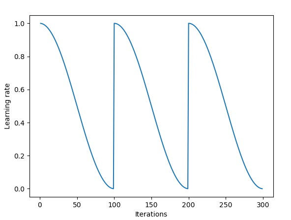
Cosine annealing 방식을 통해 학습률을 조절하였고 그에 대한 코드도 구현을 하였습니다. 우선 Cosine annealing 방식에 대해 먼저 설명을 드리면 이 방식은 “SGDR: Stochastic Gradient Descent with Warm Restarts” 라는 2017년 ICLR 논문에서 제안된 방식입니다. 위의 그림과 같이 Cosine 함수의 최고점에서 최저점으로 학습률을 감소시키고 일정 주기마다 다시 최고점으로 돌아오는(Restart) 구조를 갖고 있으며 식으로 나타내면 다음과 같습니다.
본 논문에서는 Restart를 사용하지 않고 처음부터 마지막 epoch까지 천천히 cosine 함수의 그래프를 따라 학습률을 감소시키는 방식을 사용하였고, 코드도 이 방식을 토대로 구현을 하였습니다.
(5) 학습 수행 및 테스트
train.py 에서는 실제 학습을 수행하는 과정이 구현되어 있으며 test.py 에서는 학습이 끝난 모델들을 이용하여 테스트를 수행하는 과정이 구현되어 있습니다.
train.py 스크립트
# Load training set(train_set) and test set(val_set)
X_train, X_val, Y_train, Y_val = dataset.read_CIFAR10_subset()
train_set = dataset.DataSet(X_train, Y_train)
val_set = dataset.DataSet(X_val, Y_val)

# Sanity check
print('Training set stats:')
print(train_set.images.shape)

print('Validation set stats:')
print(val_set.images.shape)

""" 2. Set training hyperparameters """
hp_d = dict()

# FIXME: Training hyperparameters
hp_d['batch_size'] = 128
hp_d['num_epochs'] = 1800

hp_d['augment_train'] = True

hp_d['init_learning_rate'] = 0.2
hp_d['momentum'] = 0.9

# FIXME: Regularization hyperparameters
hp_d['weight_decay'] = 0.0001
hp_d['dropout_prob'] = 0.0

# FIXME: Evaluation hyperparameters
hp_d['score_threshold'] = 1e-4


""" 3. Build graph, initialize a session and start training """
# Initialize
graph = tf.get_default_graph()
config = tf.ConfigProto()
config.gpu_options.allow_growth = True

model = ConvNet([32, 32, 3], 10, **hp_d)
evaluator = Evaluator()
optimizer = Optimizer(model, train_set, evaluator, val_set=val_set, **hp_d)

sess = tf.Session(graph=graph, config=config)
train_results = optimizer.train(sess, details=True, verbose=True, **hp_d)
train.py 스크립트에서는 CIFAR 10 데이터셋을 불러오고, 학습 수행 및 성능 평가와 관련된 하이퍼파라미터를 설정한 뒤, 학습을 수행하고 성능을 평가하는 역할들을 수행합니다.
- 러닝 알고리즘 관련 하이퍼 파라미터 설정
- Batch size: 128
- Number of epochs: 1800
- Initial learning rate: 0.2
- Momentum: 0.9
- 정규화 관련 하이퍼파라미터 설정
- L2 weight decay: 1e-4
- 평가 척도 관련 하이퍼파라미터 설정
- Score threshold: 1e-4
test.py 스크립트
# Load test set(val_set)
X_train, X_val, Y_train, Y_val = dataset.read_CIFAR10_subset()
train_set = dataset.DataSet(X_train, Y_train)
test_set = dataset.DataSet(X_val, Y_val)

# Sanity check
print('Test set stats:')
print(test_set.images.shape)


""" 2. Set test hyperparameters """
hp_d = dict()

# FIXME: Test hyperparameters
hp_d['batch_size'] = 128
hp_d['augment_pred'] = False

""" 3. Build graph, load weights, initialize a session and start test """
# Initialize
graph = tf.get_default_graph()
config = tf.ConfigProto()
config.gpu_options.allow_growth = True

model = ConvNet([32, 32, 3], 10, **hp_d)
evaluator = Evaluator()
saver = tf.train.Saver()

sess = tf.Session(graph=graph, config=config)
saver.restore(sess, './tmp/model.ckpt')    # restore learned weights
test_y_pred = model.predict(sess, test_set, **hp_d)
test_score = evaluator.score(test_set.labels, test_y_pred)

print('Test accuracy: {}'.format(test_score))
test.py 스크립트도 train.py 와 거의 동일한 구조로 되어있습니다. 이전 포스팅을 보셨다면 충분히 이해하실 수 있습니다.
(6) 학습 결과 분석
학습 곡선
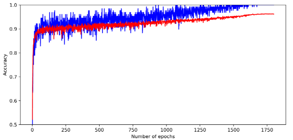
학습이 진행되면서 학습 정확도와 검증 정확도가 점차적으로 증가하는 모양을 보입니다. 그래프의 파란선이 학습 정확도를 의미하고 빨간선이 검증 정확도를 의미합니다. 학습 중 가장 검증 정확도가 높았던 모델 파라미터를 최종적으로 채택하여 checkpoint 포맷으로 저장을 하였습니다.
테스트 결과
모델을 학습 시킨 후 테스트 결과 측정된 정확도는 0.9633로 확인되었습니다. 본 논문에서 제시하고 있는 수치인 0.9645보다 낮게 측정이 되었는데 이는 지극히 정상적인 현상입니다. 같은 모델에 대해 학습을 진행하여도 Random seed를 고정하지 않는 이상 weight를 초기화할 때, mini-batch를 구성할때 등에 randomness가 개입하기 때문에 매번 약간의 성능 차이는 존재할 수 있습니다.
결론
이번 포스팅에서는 최근 주목받고 있는 Shake-Shake regularization 논문에 대해 소개를 드리고, 분석한 내용과 코드 구현체, 그에 대한 설명들을 긴 글로 작성을 하였습니다. CIFAR-10 데이터셋에서는 좋은 성능을 보임을 확인할 수 있었고, 실제 구현을 하였을 때도 비슷한 성능을 보임을 확인할 수 있었습니다. 다른 데이터셋들에 대해서는 아직 검증이 필요하지만 구현체가 같이 있으니 일부만 수정하시면 쉽게 사용 가능하리라 판단됩니다. *추후 글에서는 Shake-Shake 이후에 제안된 Cutout augmentation 기법에 대해서 소개를 드리고자 합니다. 혹시 이번 포스팅에서 이해가 잘 되시지 않는 부분은 언제든 편하게 피드백 주시면 감사하겠습니다.
Reference
- Data augmentation 예시 그림
- Shake-Shake regularization 논문
- MNIST dataset
- CIFAR-10 dataset
- drop-path 논문
- Shakeout 논문
- Whiteout 논문
- Cosine annealing learning rate decay 논문